Height Field
General introduction
A grid fluid simulation method based on a two-dimensional height field. This method represents the water surface as a continuous flat grid, and generates a series of continuous height textures corresponding to this network - called height maps. Each mesh vertex corresponds to a pixel of the height map, which is the height of the water surface, thus representing the entire water surface.
The height field fluid simulation is divided into two parts, shallow water wave simulation based on shallow water equation (SWE) and ocean wave simulation based on fast Fourier transform (FFT). The shallow water equation (SWE) is a mathematical model describing the flow of shallow water, and it is also an important mathematical model in hydraulics. The shallow water equations are based on the conservation of physical quantities with physical meaning, and can also be called hyperbolic conservation equations. The main idea of wave simulation based on fast Fourier transform (FFT) is to obtain the height field of the sea surface (that is, the frequency domain of the Fourier transform) according to the Phillips wave, and then inverse Fourier transform (IFFT) to obtain the sea surface. (aka time domain).
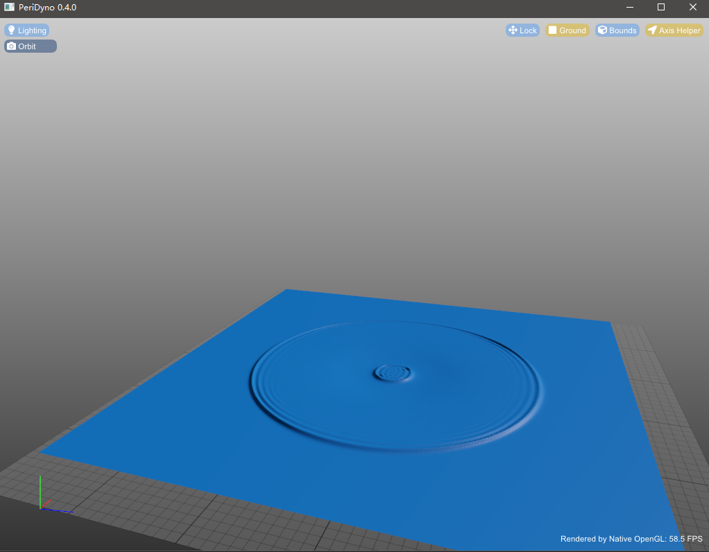
Shallow water wave simulation
At present, the Gerstner model is widely used in large-scale water simulation in real-time systems. Although Gerstner Wave is suitable for modeling large-scale water bodies, it has limited ability to display fine-scale water waves and cannot reflect the interaction of water bodies and rigid bodies. In view of this, this project uses the shallow water equation to achieve fine-scale water wave simulation:
\begin{array}{l}
\frac{{\partial h}}{{\partial t}} + \frac{\partial }{{\partial x}}\left( {hu} \right) + \frac{\partial }{{\partial y}}\left( {hv} \right) = 0 \\
\frac{\partial }{{\partial t}}\left( {hu} \right) + \frac{\partial }{{\partial x}}\left( {\frac{{h{u^2}}}{2}} \right) + \frac{\partial }{{\partial y}}\left( {huv} \right) = - gh\frac{{\partial s}}{{\partial x}} \\
\frac{\partial }{{\partial t}}\left( {hv} \right) + \frac{\partial }{{\partial x}}\left( {huv} \right) + \frac{\partial }{{\partial y}}\left( {\frac{{h{v^2}}}{2}} \right) = - gh\frac{{\partial s}}{{\partial y}}
\end{array}
Among them, u and v represent the two components of the horizontal velocity of the ocean current, h represents the depth of the ocean current, s represents the vertical coordinate of the sea surface, and g represents the acceleration of gravity. In the solution process, the simulation area is firstly discretized based on the height field as shown in the figure below.
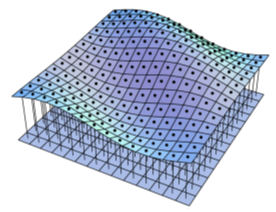
Then, the position of the height field at each moment is calculated by solving the wave equation. Finally, the height field based on the shallow water equation (SWE) is superimposed on the large area water body to achieve a more realistic water body simulation.
First initialize the initial height of the water surface. For the height of the water surface boundary, after each calculation:
a) The height value of the particle at point x=0 is equal to the height value of the particle at point x=1;

b) The particle height value of x= width - 1 point is equal to the particle height value of x= width - 2 points;

c) The particle height value at y=0 point is equal to the particle height value at y=1 point;

d) The height of the particle at y= height- 1 is equal to the height of the particle at y= height - 2.
参考代码src\Dynamics\HeightField\CapillaryWave.cu。
__global__ void C_ImposeBC(Vec4f* grid_next, Vec4f* grid, int width, int height, int pitch)
	{
		int x = threadIdx.x + blockIdx.x * blockDim.x;
		int y = threadIdx.y + blockIdx.y * blockDim.y;
		if (x < width && y < height)
		{
			if (x == 0)
			{
				Vec4f a = grid[(y)*pitch + 1];
				grid_next[(y)*pitch + x] = a;
			}
			else if (x == width - 1)
			{
				Vec4f a = grid[(y)*pitch + width - 2];
				grid_next[(y)*pitch + x] = a;
			}
			else if (y == 0)
			{
				Vec4f a = grid[(1) * pitch + x];
				grid_next[(y)*pitch + x] = a;
			}
			else if (y == height - 1)
			{
				Vec4f a = grid[(height - 2) * pitch + x];
				grid_next[(y)*pitch + x] = a;
			}
			else
			{
				Vec4f a = grid[(y)*pitch + x];
				grid_next[(y)*pitch + x] = a;
			}
		}
	}
Iterate over the height field at each time:
  __global__ void C_OneWaveStep(Vec4f* grid_next, Vec4f* grid, int width,
  int height, float timestep, int pitch)
Finally, calculate the two components of the horizontal velocity of the u and v ocean currents, the depth of the h ocean current, and the s vertical coordinate of the sea surface.
__global__ void C_InitHeightField(
		Vec4f* height,
		Vec4f* grid,
		int patchSize,
		float horizon,
		float realSize)
	{
		int i = threadIdx.x + blockIdx.x * blockDim.x;
		int j = threadIdx.y + blockIdx.y * blockDim.y;
		if (i < patchSize && j < patchSize)
		{
			int gridx = i + 1;
			int gridy = j + 1;

			Vec4f gp = grid[gridx + patchSize * gridy];
			height[i + j * patchSize].x = gp.x - horizon;

			float d = sqrtf((i - patchSize / 2) * (i - patchSize / 2) + (j - patchSize / 2) * (j - patchSize / 2));
			float q = d / (0.49f * patchSize);

			float weight = q < 1.0f ? 1.0f - q * q : 0.0f;
			height[i + j * patchSize].y = 1.3f * realSize * sinf(3.0f * weight * height[i + j * patchSize].x * 0.5f * M_PI);
		}
	}
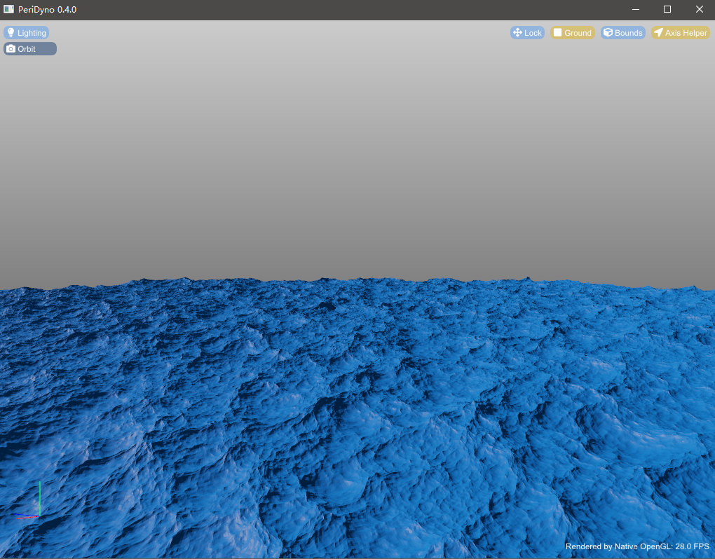
Wave Simulation Based on Fast Fourier Transform (FFT)
The FFT model is a statistical model. Unlike the Gerstner model, which uses multiple sine and cosine functions to fit, the FFT model uses Fourier transform. The core of Fourier transform is to use sin(nx) and cos(nx) to simulate any periodic function. In the FFT model, the wave height is represented by a random function h(x,t) of time and level. This method has high simulation degree and is easy to model, and its calculation formula is as follows[1]:
$$h(X,t) = \sum\limits_K^{} {\tilde h(K,t){{\mathop{\rm e}\nolimits} ^{(iK{\rm{X}})}}} $$
In the formula, $X{\rm{ = }}(x, z)$ horizontal position; $t$ represents time; $K$ is a two-dimensional vector; $\tilde h(k,t)$ represents the surface structure of waves .
After building the height field of the FFT model, the next step is to create a random height field. Introduce a Gaussian random function, as follows:
$${\tilde h_0}(K) = \frac{1}{{\sqrt 2 }}({\xi _r} + i{\xi _i})\sqrt {{P_h}(K)} $$
Among them, ${\xi _r}$ and ${\xi _i}$ are independent Gaussian random numbers (mean 0, variance 1). At this time, the amplitude of the wave at time $t$ is:
$$\tilde h(K,t) = \tilde h(K){e^{i\omega (K)t}} + \tilde h_0^*( - K){e^{ - i\omega ({\rm{K}})t}}$$
Among them, $\omega (k)$ is the angular frequency of the wave $K$, which can be calculated according to ${\omega ^2}(k) = g|K|$; the * sign represents the conjugate operation of complex numbers. According to the FFT model, the height of the ocean wave must eventually be a real number, so it must satisfy $\tilde h(-K)= \tilde h_0^*(K)$.
template<typename TDataType>
void OceanPatch<TDataType>::generateH0(Vec2f* h0)
{
    for (unsigned int y = 0; y <= mResolution; y++)
    {
        for (unsigned int x = 0; x <= mResolution; x++)
        {
            float kx = (-( int )mResolution / 2.0f + x) * (2.0f * CUDART_PI_F / m_realPatchSize);
            float ky = (-( int )mResolution / 2.0f + y) * (2.0f * CUDART_PI_F / m_realPatchSize);

            float P = sqrtf(phillips(kx, ky, windDir, m_windSpeed, A, dirDepend));

            if (kx == 0.0f && ky == 0.0f)
            {
                P = 0.0f;
            }
            float Er = gauss();
            float Ei = gauss();

            float h0_re = Er * P * CUDART_SQRT_HALF_F;
            float h0_im = Ei * P * CUDART_SQRT_HALF_F;

            int i   = y * mSpectrumWidth + x;
            h0[i].x = h0_re;
            h0[i].y = h0_im;
        }
    }
}
Initialize phase and amplitude. The spectrum can be the Phillips spectrum. Phillips spectrum is suitable for parallelized computation of sea surface grids. It is a more realistic spectrum and is mostly used under the influence of wind. The Phillips spectrum is defined as follows:
$${P_h}(K) = A\frac{{\exp ( - 1/{{(kL)}^2})}}{{{k^4}}}|\hat K\hat \omega {|^2}$$
Among them, $g$ represents the acceleration of gravity; $k = |K| = 2\pi / \lambda $; $\lambda $ represents the wavelength; $A$ represents a constant coefficient; $L = {V^2}/g$ Represents the maximum wave generated by the wind speed in the case of $V$; $\hat \omega $ represents the wind direction; $|\hat K\hat \omega {|^2}$ represents the elimination of waves that move perpendicular to the wind direction.
// generate wave heightfield at time t based on initial heightfield and dispersion relationship
__global__ void generateSpectrumKernel(Vec2f*      h0,
                                       Vec2f*      ht,
                                       unsigned int in_width,
                                       unsigned int out_width,
                                       unsigned int out_height,
                                       float        t,
                                       float        patchSize)
{
    unsigned int x         = blockIdx.x * blockDim.x + threadIdx.x;
    unsigned int y         = blockIdx.y * blockDim.y + threadIdx.y;
    unsigned int in_index  = y * in_width + x;
    unsigned int in_mindex = (out_height - y) * in_width + (out_width - x);  // mirrored
    unsigned int out_index = y * out_width + x;

    // calculate wave vector
    Vec2f k;
    k.x = (-( int )out_width / 2.0f + x) * (2.0f * CUDART_PI_F / patchSize);
    k.y = (-( int )out_width / 2.0f + y) * (2.0f * CUDART_PI_F / patchSize);

    // calculate dispersion w(k)
    float k_len = sqrtf(k.x * k.x + k.y * k.y);
    float w     = sqrtf(9.81f * k_len);

    if ((x < out_width) && (y < out_height))
    {
        Vec2f h0_k  = h0[in_index];
        Vec2f h0_mk = h0[in_mindex];

        // output frequency-space complex values
        ht[out_index] = complex_add(complex_mult(h0_k, complex_exp(w * t)), complex_mult(conjugate(h0_mk), complex_exp(-w * t)));
        //ht[out_index] = h0_k;
    }
}
In the process of fluid simulation using the FFT model, the normal vector of the surface needs to be calculated from the slope of each point. In the actual calculation process, the finite difference of adjacent grid points is generally used to calculate the slope value. However, in order to reduce the slope error of the wavelet wavelength, the inverse FFT transformation can be used to solve:
$$\nabla h(X,t) = \sum\limits_K^{} {iK\tilde h(K,t)\exp (iKX)} $$
  cufftExecC2C(fftPlan, (float2*)m_ht, (float2*)m_ht, CUFFT_INVERSE);
  cufftExecC2C(fftPlan, (float2*)m_Dxt, (float2*)m_Dxt, CUFFT_INVERSE);
  cufftExecC2C(fftPlan, (float2*)m_Dzt, (float2*)m_Dzt, CUFFT_INVERSE);
In addition, a bias vector D(x,t) is needed to simulate the wave tip of seawater, which can be set as follows:
$$D(x,t) = \sum\limits_k { - i\frac{k}{{|k|}}h(k,t){e^{ikx}}} $$
where the Jacobian matrix is:
\begin{equation}
J\left( x \right) =\left| \begin{matrix}
J_{xx}& J_{xy}\\
J_{zx}& J_{yy}\\
\end{matrix} \right|
\end{equation}
$$
\begin{array}{l}
J_{xx}=\frac{\partial x^{'}}{\partial x}=1+\lambda \frac{\partial D_x\left( x,t \right)}{\partial x}\\
J_{yy}=\frac{\partial y^{'}}{\partial y}=1+\lambda \frac{\partial D_y\left( x,t \right)}{\partial y}\\
J_{yx}=\frac{\partial y^{'}}{\partial x}=\lambda \frac{\partial D_y\left( x,t \right)}{\partial x}\\
J_{xy}=\frac{\partial x^{'}}{\partial y}=\lambda \frac{\partial D_x\left( x,t \right)}{\partial y}\\
\end{array}
$$
References
[1] Tessendorf J. Simulating ocean water[J]. Simulating nature: realistic and interactive techniques. SIGGRAPH, 2001, 1(2): 5.